[Case1] Boston Housing Price Dataset
0) Set Random Seed for Later Reproducibility
#https://keras.io/ko/getting-started/faq/#how-can-i-obtain-reproducible-results-using-keras-during-development

import numpy as np
import tensorflow as tf
import random as rn
np.random.seed(42) # For starting core Python generated random numbers
rn.seed(12345) # Random number generation in the TensorFlow backend
tf.random.set_seed(1234) # Random number generation in the TensorFlow backend
1) Loading the Boston housing dataset
#https://keras.io/api/datasets/boston_housing/#load_data-function
#tf.keras.datasets.boston_housing.load_data(
#    path="boston_housing.npz", test_split=0.2, seed=113)
# feature, target: median values of the houses in $1,000.
from tensorflow.keras.datasets import boston_housing
(train_ft, train_tg), (test_ft, test_tg) = boston_housing.load_data()
print(f'train:test={len(train_ft)}:{len(test_ft)}')
train:test=404:102
2) Normalizing the data
# m=[[1,2],     +----> axis=1
#    [3,4]]    |
#             axis=0
ft_wise_mean = train_ft.mean(axis=0) # feature-wise mean
train_ft -= ft_wise_mean
ft_wise_std = train_ft.std(axis=0) # feature-wise std
train_ft /= ft_wise_std
#
test_ft -= ft_wise_mean
test_ft /= ft_wise_std
3) Model definition
num_features = len(train_ft[1])
num_features # 13
from tensorflow.keras.models import Sequential
from tensorflow.keras.layers import Dropout, Dense
def build_regression_model():
    model = Sequential()
    model.add( Dense(64, activation='relu') )
    model.add( Dense(64, activation='relu') )
    model.add( Dense(1) )
    model.compile(optimizer='rmsprop', loss='mse', metrics=['mae'])
    return model
4) K-fold validation + Saving the validation logs at each fold
all_mae_trace = []
def k_fold_validation(k, num_epochs, num_batch):
    all_val_scores = []
    val_samples = len(train_ft)//k
    for i in range(k):
# 1) prepare validation data from partition k
        val_ft_k = train_ft[i*val_samples : (i+1)*val_samples]
        val_tg_k = train_lb[i*val_samples : (i+1)*val_samples]
# 2) prepare training data
        train_ft_k = np.concatenate(
        [ train_ft[:i*val_samples], train_ft[(i+1)*val_samples:] ],
        axis=0) # feature-wise, i.e. column-wise
        train_tg_k = np.concatenate(
        [ train_tg[:i*val_samples], train_tg[(i+1)*val_samples:] ],
        axis=0) # feature-wise, i.e. column-wise
# 3) build keras model
        model = build_regression_model()
        ################################
# 4) train model
        trace = model.fit(train_ft_k, train_tg_k,
            validation_data=(val_ft_k, val_tg_k), ### k-fold val
            epochs=num_epochs,
            batch_size=num_batch, verbose=0)
# 5) evaluate model on the validation set
        val_mse, val_mae = model.evaluate(
            val_ft_k, val_tg_k, verbose=0)
        all_val_scores.append(val_mae)
    all_mae_trace.append(trace.history['val_mae'])
    return all_val_scores
5) Building the history of successive mean K-fold validation scores
k, num_epochs, num_batch = 4, 100, 20
k_fold_validation(k, num_epochs, num_batch)
avg_mae_trace = [np.mean([x[i] for x in all_mae_trace]) \
                 for i in range(num_epochs)]
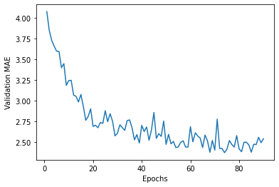
6) Plotting validation scores
import matplotlib.pyplot as plt
avg_mae_trace = avg_mae_trace[10:]
plt.plot(range(1, len(avg_mae_trace)+1), avg_mae_trace)
plt.xlabel('Epochs')
plt.ylabel('Validation MAE')
Text(0, 0.5, 'Validation MAE')

8) Fianl Training, Evaluation and Prediction
# final training
model = build_regression_model()
model.fit(train_ft, train_tg,
          epochs=130, batch_size=16, verbose=0)

# evaluate
test_mse_loss, test_mae_score = model.evaluate(test_ft, test_tg,
                                              verbose=0)
print(f'Mean Abs Error = ${test_mae_score*1000:.2f}')

# predict
predict_vec = model.predict(test_ft)
predict_diff = np.array([abs(p-test_tg[i]) \
                         for i, p in enumerate(predict_vec)])
print(f'Mean Abs Error = ${predict_diff.mean()*1000:.2f}')
Mean Abs Error = $2442.92
Mean Abs Error = $2442.92
[Case2] Hyderabad Housing Price Dataset
0) For reproducibility, set random seed as a practice
import numpy as np
import tensorflow as tf
SEED=1
np.random.seed(SEED)
tf.random.set_seed(SEED)
1) Loading, preprocessing regression dataset
import pandas as pd
data = pd.read_csv('Hyderabad.csv')
data.head()
| Price | Area | Location | No. of Bedrooms | Resale | MaintenanceStaff | Gymnasium | SwimmingPool | LandscapedGardens | JoggingTrack | ... | LiftAvailable | BED | VaastuCompliant | Microwave | GolfCourse | TV | DiningTable | Sofa | Wardrobe | Refrigerator | |
|---|---|---|---|---|---|---|---|---|---|---|---|---|---|---|---|---|---|---|---|---|---|
| 0 | 6968000 | 1340 | Nizampet | 2 | 0 | 0 | 1 | 1 | 1 | 1 | ... | 1 | 0 | 1 | 0 | 0 | 0 | 0 | 0 | 0 | 0 |
| 1 | 29000000 | 3498 | Hitech City | 4 | 0 | 0 | 1 | 1 | 1 | 1 | ... | 1 | 0 | 1 | 0 | 0 | 0 | 0 | 0 | 0 | 0 |
| 2 | 6590000 | 1318 | Manikonda | 2 | 0 | 0 | 1 | 0 | 0 | 0 | ... | 0 | 0 | 0 | 0 | 0 | 0 | 0 | 0 | 0 | 0 |
| 3 | 5739000 | 1295 | Alwal | 3 | 1 | 0 | 0 | 0 | 0 | 0 | ... | 1 | 0 | 0 | 0 | 0 | 0 | 0 | 0 | 0 | 0 |
| 4 | 5679000 | 1145 | Kukatpally | 2 | 0 | 0 | 0 | 0 | 1 | 0 | ... | 1 | 0 | 0 | 0 | 0 | 0 | 0 | 0 | 0 | 0 |
5 rows × 40 columns
!pip install scikit-learn
Requirement already satisfied: scikit-learn in /opt/anaconda3/envs/KerasPy3.6/lib/python3.6/site-packages (0.24.2)
Requirement already satisfied: numpy>=1.13.3 in /opt/anaconda3/envs/KerasPy3.6/lib/python3.6/site-packages (from scikit-learn) (1.19.5)
Requirement already satisfied: threadpoolctl>=2.0.0 in /opt/anaconda3/envs/KerasPy3.6/lib/python3.6/site-packages (from scikit-learn) (2.1.0)
Requirement already satisfied: scipy>=0.19.1 in /opt/anaconda3/envs/KerasPy3.6/lib/python3.6/site-packages (from scikit-learn) (1.5.4)
Requirement already satisfied: joblib>=0.11 in /opt/anaconda3/envs/KerasPy3.6/lib/python3.6/site-packages (from scikit-learn) (1.0.1)
targets = data['Price'] # ground-truth to be predicted
features = data.drop(['Price', 'Location'], axis=1) # column

# normalize data
features_mean = features.mean(axis=0) # feature-wise mean
features -= features_mean
features_std = features.std(axis=0) # feature-wise std
features /= features_std

from sklearn.model_selection import train_test_split
# spilt data into train:test=8:2
train_ft, test_ft, train_tg, test_tg =\
train_test_split(features, targets, test_size=0.2)
train_ft = train_ft.to_numpy()
train_tg = train_tg.to_numpy()
test_ft = test_ft.to_numpy()
test_tg = test_tg.to_numpy()
print(f'train:test={len(train_ft)/len(test_ft):.2f}')
train:test=4.00
2) Building a regression model
# build a model
from tensorflow.keras.models import Sequential
from tensorflow.keras.layers import Dense, Dropout
ncols = features.shape[1]
model =  Sequential()
model.add( Dense(ncols, activation='relu', input_shape=(ncols,)) )
model.add( Dropout(0.2) )
model.add( Dense(128, activation='relu') )
model.add( Dropout(0.2) )
model.add( Dense(64, activation='relu') )
model.add( Dropout(0.2) )
model.add( Dense(1) ) # output = no activation
3) Training
# compile a model with specific optimizer, loss, and monitoring metric
model.compile(optimizer='rmsprop', loss='mse', metrics=['mae'])
# training with dataset, epochs, and batch_size
model.fit(train_ft, train_tg, epochs=50, batch_size=10, verbose=0)
<tensorflow.python.keras.callbacks.History at 0x153b64fd0>
4) Evaluation (loss), Prediction (final answer)
# evaluate
test_mse_loss, test_mae_score = model.evaluate(test_ft, test_tg,
                                              verbose=0)
print(f'Mean Abs Error = ${test_mae_score:.2f}')

# predict
predictions = model.predict(test_ft)
predict_diff = np.array([abs(p-test_tg[i]) \
                         for i, p in enumerate(predictions)])
print(f'Mean Abs Error = ${predict_diff.mean():.2f}')
Mean Abs Error = $2294626.25
Mean Abs Error = $2294626.05